📘 Test Statistic & Standardized Testing Logic

A test statistic is a standardized numerical value that measures how far a sample result deviates from what is expected under the null hypothesis.

It converts sample evidence into a measurable scale so we can evaluate whether the result is unusual.

🎯 Why Test Statistics are Needed

When we collect sample data, the result rarely matches the population value exactly due to sampling variability.

We must determine whether the difference is:

Small → due to random variation
Large → evidence against the null hypothesis

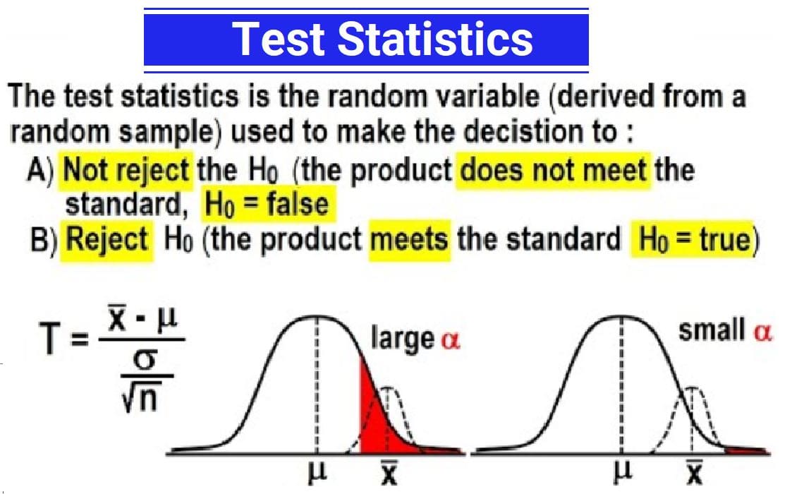
A test statistic helps quantify "how large" the difference is.

📏 General Structure of a Test Statistic

\[ \text{Test Statistic} = \frac{\text{Observed Value} - \text{Expected Value}}{\text{Standard Error}} \]

This measures how many standard errors the sample result is away from the null hypothesis value.

It expresses deviation in standardized units.

🧠 Conceptual Meaning

Small test statistic → Sample close to expectation
Large test statistic → Sample far from expectation

Larger deviations make the null hypothesis less believable.

📐 Standardization Principle

Standardization converts different measurement scales into a common scale.

This allows comparison using probability distributions.

Just like z-scores standardize observations, test statistics standardize evidence.

🔢 Common Test Statistics

1️⃣ Z-Test Statistic (Known σ or Large Sample)

\[ Z = \frac{\bar{x} - \mu_0}{\sigma / \sqrt{n}} \]

Used when population standard deviation is known
Used for large samples

2️⃣ t-Test Statistic (Unknown σ)

\[ t = \frac{\bar{x} - \mu_0}{s / \sqrt{n}} \]

Uses sample standard deviation
Used for small samples

3️⃣ Proportion Z-Test

\[ Z = \frac{\hat{p} - p_0}{\sqrt{p_0(1-p_0)/n}} \]

Used for binary outcomes
Common in surveys and classification accuracy

🔍 Example 1 — Mean Test

Claim: Average battery life is 10 hours

Sample Data:

Sample mean = 11 hours
Population σ = 2 hours
Sample size = 100

Step 1: Standard Error

\[ SE = \frac{2}{\sqrt{100}} = \frac{2}{10} = 0.2 \]

Step 2: Test Statistic

\[ Z = \frac{11 - 10}{0.2} = \frac{1}{0.2} = 5 \]

The sample mean is 5 standard errors above the claimed mean → Strong evidence.

🔍 Example 2 — Proportion Test

Claim: Defect rate is 5%

Sample Data:

Sample proportion = 8%
Sample size = 400

Test Statistic

\[ Z = \frac{0.08 - 0.05}{\sqrt{0.05(0.95)/400}} = \frac{0.03}{\sqrt{0.00011875}} = \frac{0.03}{0.0109} \approx 2.75 \]

Observed defect rate is 2.75 standard errors above expected.

📊 Interpreting Test Statistics

Test Statistic Value	Interpretation
Near 0	Data consistent with H₀
Moderate	Some evidence against H₀
Large	Strong evidence against H₀

🎯 Critical Regions

If the test statistic falls in extreme regions of the probability distribution, we reject H₀.

Extreme deviations are unlikely under the null hypothesis.

🔗 Link with p-value

The test statistic determines the p-value.

Larger test statistic → Smaller p-value
Smaller p-value → Stronger evidence

🤖 Importance in Machine Learning

Comparing algorithm performance
Evaluating model improvements
Feature selection testing
A/B testing systems

Test statistics quantify improvement significance.

🧠 Key Insights

Test statistic standardizes sample evidence
Measures deviation from null hypothesis
Expressed in standard error units
Forms basis for probability-based decisions
Used to compute p-values

Test Statistic & Standardized Testing Logic