📊 Sampling and Population in Statistical Estimation
In most real-world situations, studying an entire population is impractical due to limitations of time, cost, or accessibility. Sampling provides an efficient and scientifically valid alternative.
👥 Population
A population is the complete set of individuals, objects, or measurements that share a common characteristic being studied.
Examples
- All citizens of a country
- All students in a university
- All manufactured light bulbs in a factory
- All patients with a specific disease
Common population parameters include:
- μ (mu) — population mean
- σ (sigma) — population standard deviation
- p — population proportion
🔍 Sample
A sample is a subset of the population selected for study.
Samples are used to estimate population parameters.
Common sample statistics include:
- x̄ — sample mean
- s — sample standard deviation
- p̂ — sample proportion
🎯 Purpose of Sampling
- Reduce cost and time of data collection
- Make population estimation feasible
- Enable scientific inference
- Allow probability-based modeling
🧮 Example 1 — Estimating a Population Proportion (Categorical Variable)
Suppose researchers study whether individuals have a particular disease.
A random sample of 100 people is selected.
Among them, 12 people are found to have the disease.
Sample Proportion
\[ \hat{p} = \frac{12}{100} = 0.12 \]
This means that in the sample, 12% of individuals have the disease.
This value is used to estimate the true population proportion p.
📊 Sample Distribution (Categorical Data)
The sample information can be displayed using a bar chart showing:
- Probability of disease = 0.12
- Probability of no disease = 0.88
This graphical summary represents the distribution of the sample data.
🌍 Population Distribution (Theoretical Model)
Suppose medical records reveal that in the entire population, the true disease rate is:
p = 0.10 (10%)
This population behavior can be modeled using a probability distribution.
The binomial model describes:
- Number of trials (n)
- Probability of success (p)
Thus, population behavior is described theoretically, while sample behavior is observed empirically.
🧮 Example 2 — Estimating a Population Mean (Numerical Variable)
Suppose a researcher studies the heights of individuals.
A random sample of 100 individuals is collected.
Height is a numerical variable.
Sample Statistics Computed
- Sample Mean = x̄
- Sample Standard Deviation = s
The distribution of sample heights can be displayed using:
- Histogram
- Box plot
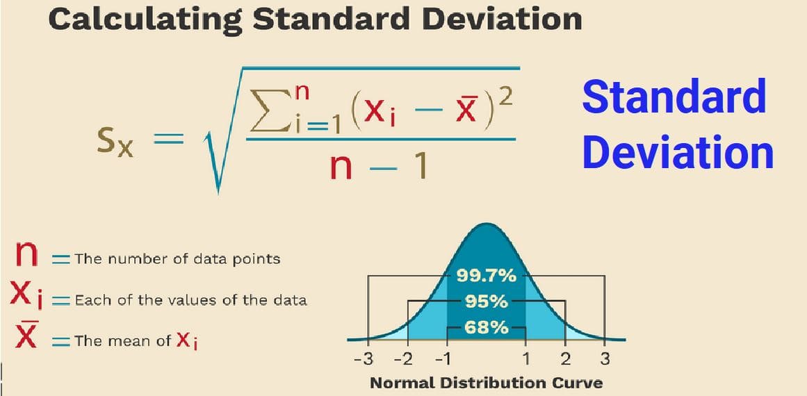
🌍 Population Distribution for Numerical Data
Suppose demographic studies reveal:
- True mean height μ = 175 cm
- True standard deviation σ = 10 cm
- Heights are approximately normally distributed
This population behavior is modeled using the Normal Distribution.
Population models help predict how sample statistics behave.
🔁 Connecting Sample and Population
| Aspect | Sample | Population |
|---|---|---|
| Scope | Subset | Entire group |
| Measures | Statistics | Parameters |
| Mean | x̄ | μ |
| Std. Deviation | s | σ |
| Proportion | p̂ | p |
| Distribution | Empirical | Theoretical |
🎯 Why Sampling Works
If samples are randomly selected:
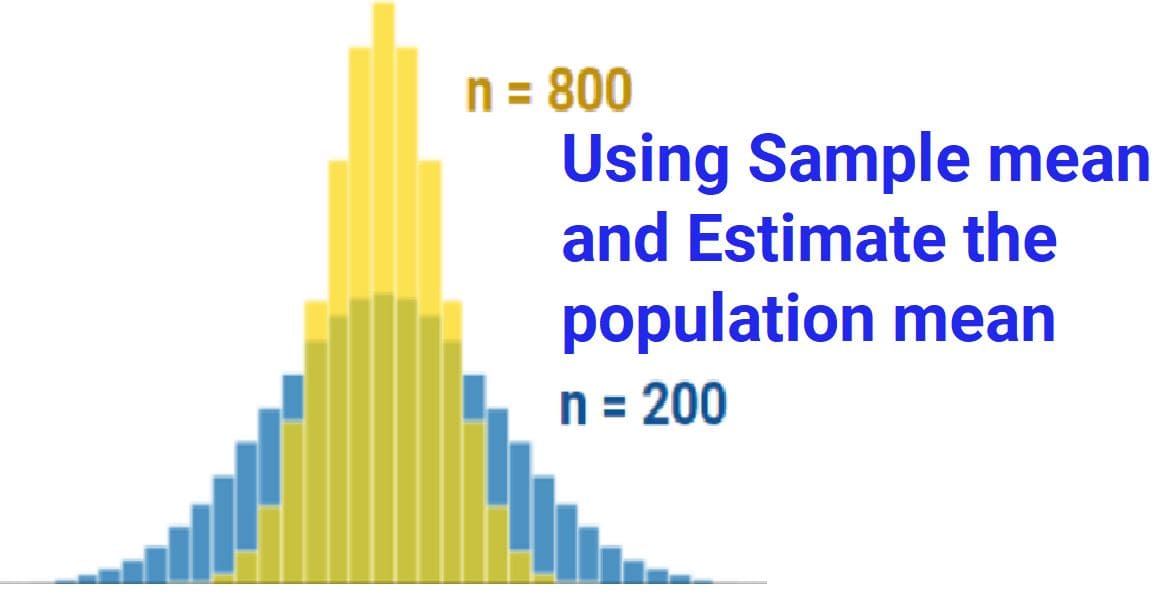
- They tend to reflect population characteristics
- Sample statistics cluster around population parameters
- Larger samples give more accurate estimates
🌍 Real-World Applications
- Election polling
- Public health surveys
- Market research
- Quality testing in manufacturing
- Machine learning model training
🧠 Key Insights
- Populations contain all individuals of interest
- Samples are subsets used for analysis
- Statistics estimate unknown parameters
- Probability distributions model population behavior
- Sampling enables reliable estimation and prediction