📊 Sampling Distribution of the Mean
It is a theoretical probability distribution that forms the foundation of statistical inference.
🎯 Why It Is Important
When we collect a sample, the sample mean is unlikely to be exactly equal to the population mean.
Different random samples produce different sample means.
It helps us measure estimation uncertainty and forms the basis for confidence intervals and hypothesis testing.
👥 Population vs Samples
Consider a population with many individuals.
If we repeatedly draw samples of equal size and compute their means, we obtain many sample means.
🧮 Illustrative Example
Suppose a small population consists of five values:
2, 4, 6, 8, 10
Population mean:
\[ \mu = \frac{2+4+6+8+10}{5} = 6 \]
Now consider all possible samples of size 2.
| Sample | Sample Mean |
|---|---|
| (2,4) | 3 |
| (2,6) | 4 |
| (2,8) | 5 |
| (2,10) | 6 |
| (4,6) | 5 |
| (4,8) | 6 |
| (4,10) | 7 |
| (6,8) | 7 |
| (6,10) | 8 |
| (8,10) | 9 |
These sample means form a new distribution.
📈 Properties Observed
1️⃣ Mean of Sampling Distribution
The average of all sample means equals the population mean.
Mean of sample means = 6 = μ
2️⃣ Spread Is Smaller
Sample means vary less than individual data values.
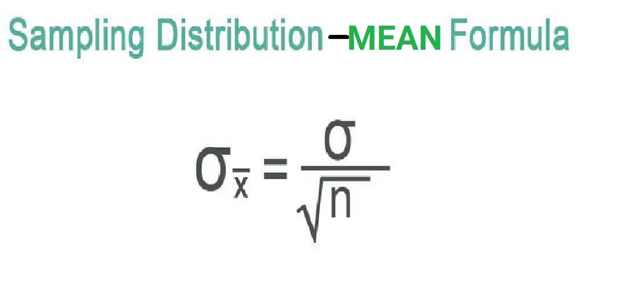
📐 Standard Error of the Mean
The spread of the sampling distribution is measured by the Standard Error (SE).
\[ SE = \frac{\sigma}{\sqrt{n}} \]
- σ = population standard deviation
- n = sample size
🧠 Key Properties
| Property | Result |
|---|---|
| Mean | Equals population mean (μ) |
| Spread | σ / √n (Standard Error) |
| Shape | Approximately normal for large samples |
📏 Effect of Sample Size
As sample size increases:
- Standard error decreases
- Estimates become more stable
- Distribution becomes more concentrated around μ
🔔 Connection to Central Limit Theorem
Even if the population is not normally distributed:
This powerful result is known as the Central Limit Theorem.
🧮 Practical Example
Population mean exam score μ = 70 Population standard deviation σ = 12 Sample size n = 36
Standard Error
\[ SE = \frac{12}{\sqrt{36}} = \frac{12}{6} = 2 \]
📊 Interpretation
If many samples of 36 students are taken:
- Most sample means will lie close to 70
- Very large deviations are unlikely
- The distribution of sample means is normal
🌍 Real-Life Applications
🏥 Medicine
- Estimating average treatment effects
📘 Education
- Estimating average performance of students
🏭 Manufacturing
- Estimating average product quality
💹 Economics
- Estimating national income averages
🤖 Artificial Intelligence
- Model evaluation using batch averages
- Mini-batch gradient descent
- Performance estimation
🧠 Why This Concept Matters
- Explains why sample estimates fluctuate
- Quantifies estimation uncertainty
- Foundation for confidence intervals
- Foundation for hypothesis testing
- Core principle behind AI model reliability