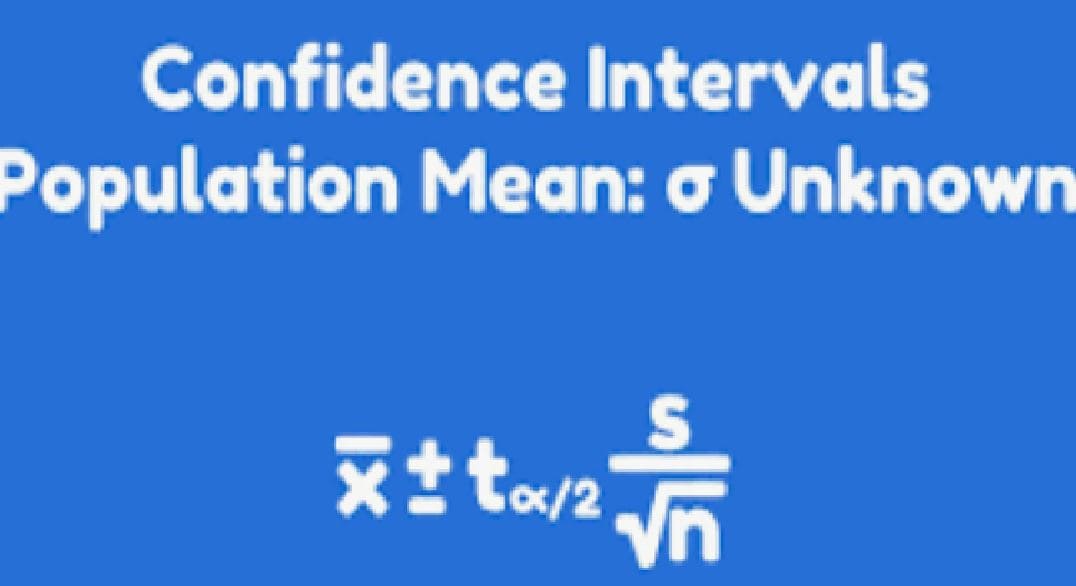
📘 Confidence Interval for Population Mean (σ Unknown)

When the population standard deviation (σ) is unknown, we estimate it using the sample standard deviation (s) and use the Student’s t-distribution instead of the normal (Z) distribution.

This situation is more realistic because population variability is rarely known in practical studies.

🎯 Objective

To estimate the true population mean (μ) when population variability is unknown.

We account for extra uncertainty by using the t-distribution.

📐 Why Not Use Z-Distribution?

When σ is unknown, replacing it with sample standard deviation (s) introduces additional estimation error.

Sample standard deviation varies from sample to sample
This adds extra uncertainty
Z-distribution underestimates this uncertainty

The t-distribution adjusts for this added variability.

📊 Properties of the t-Distribution

Bell-shaped and symmetric (like normal distribution)
Has heavier tails (more spread)
Accounts for extra uncertainty in estimating σ
Shape depends on Degrees of Freedom (df)

As sample size increases, the t-distribution approaches the normal distribution.

📏 Degrees of Freedom

Degrees of Freedom (df) measure the number of independent values used to estimate variability.

\[ df = n - 1 \]

n = sample size

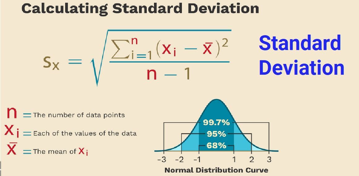
Smaller samples → smaller df → wider t-distribution → larger margin of error

📊 Standard Error (Estimated)

Since σ is unknown, we estimate Standard Error using sample standard deviation:

\[ SE = \frac{s}{\sqrt{n}} \]

📐 Formula for Confidence Interval

\[ \bar{x} \pm t_{\alpha/2, df} \cdot \frac{s}{\sqrt{n}} \]

Where:

x̄ = Sample Mean
t = t-score from t-table
s = Sample Standard Deviation
n = Sample Size
df = n − 1

🔢 Example 1: Estimating Average Battery Life

Given:

Sample mean battery life = 10 hours
Sample standard deviation = 2 hours
Sample size = 25
Confidence level = 95%

Step 1: Degrees of Freedom

df = 25 − 1 = 24

Step 2: Standard Error

\[ SE = \frac{2}{\sqrt{25}} = \frac{2}{5} = 0.4 \]

Step 3: t-value

From t-table for 95% confidence and df = 24:

t ≈ 2.064

Step 4: Margin of Error

\[ ME = 2.064 \times 0.4 = 0.826 \]

Step 5: Construct Interval

10 ± 0.826

Confidence Interval = (9.174 hours, 10.826 hours)

📊 Interpretation

We are 95% confident that the true average battery life lies between 9.174 and 10.826 hours.

The wider interval reflects added uncertainty from estimating σ.

⚖️ t-Distribution vs Normal Distribution

Feature	Z-Distribution	t-Distribution
Population SD	Known	Unknown
Spread	Narrower	Wider
Tail Thickness	Thin tails	Heavy tails
Depends on df?	No	Yes

📈 When to Use t-Distribution

Population standard deviation unknown
Sample size small (n < 30)
Population approximately normal
Random and independent sampling

🤖 Applications in Machine Learning

Estimating true model performance with small validation sets
Evaluating uncertainty in experimental results
Comparing algorithms using limited data
Estimating real-world prediction accuracy

The t-distribution allows reliable estimation even with limited data.

🧠 Key Insights

Use t-distribution when σ is unknown
Degrees of freedom control shape of distribution
Smaller samples → larger uncertainty
Interval is wider than Z-interval
t-distribution approaches normal for large samples

Confidence Interval for Population Mean (σ Unknown)