📊 Central Limit Theorem (CLT)
It is one of the most powerful and important results in statistics because it explains why the normal distribution appears so frequently in real-world data analysis.
🎯 Why the Central Limit Theorem Matters
- Allows probability calculations for sample means
- Enables statistical inference
- Supports estimation and hypothesis testing
- Justifies use of normal distribution in many situations
🧠 Conceptual Understanding
Individual observations from a population may not follow a normal distribution.
However, when we repeatedly take samples and compute their means:
This happens even if the original population is skewed or irregular.
📐 Formal Statement of CLT
If samples of size n are randomly drawn from any population with:
- Population mean = μ
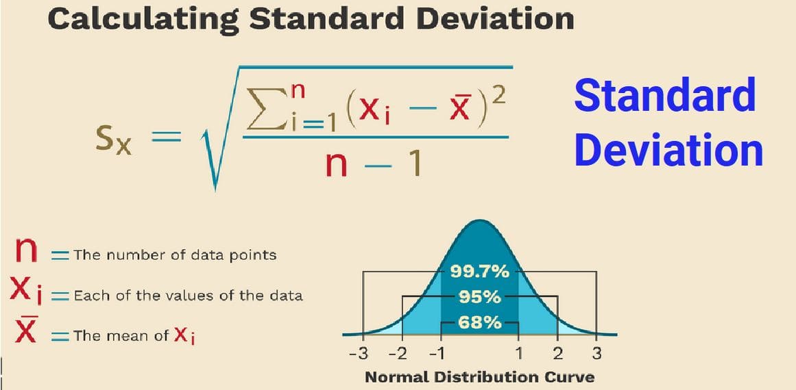
- Population standard deviation = σ
Then for sufficiently large n:
- The mean of sample means = μ
- The standard deviation of sample means = σ / √n
- The sampling distribution approaches normality
📏 Conditions for Central Limit Theorem
- Samples must be randomly selected
- Observations should be independent
- Sample size should be sufficiently large (typically n ≥ 30)
🧮 Intuitive Illustration
Consider rolling a fair die.
Single roll outcomes are not normally distributed; they are discrete and uniform.
Now suppose we:
- Roll the die 30 times
- Compute the average of the 30 outcomes
- Repeat this process many times
📊 Visual Behavior as Sample Size Increases
| Sample Size | Shape of Sampling Distribution |
|---|---|
| Small (n < 10) | Irregular, resembles population |
| Moderate (10 ≤ n < 30) | Becoming smoother |
| Large (n ≥ 30) | Approximately normal |
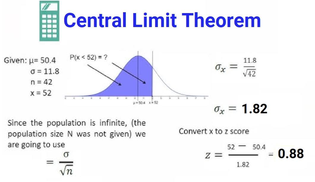
🧮 Numerical Example
Suppose a population has:
- Mean μ = 50
- Standard deviation σ = 12
A sample of size n = 36 is drawn.
Sampling Distribution Properties
Mean of sample means:
μx̄ = μ = 50
Standard Error:
\[ SE = \frac{σ}{\sqrt{n}} = \frac{12}{\sqrt{36}} = \frac{12}{6} = 2 \]
📈 Practical Interpretation
If many samples of size 36 are taken:
- Most sample means will be close to 50
- Few will be far from 50
- The distribution of sample means will be bell-shaped
🔗 Relationship with Normal Distribution
CLT explains why the normal distribution is widely applicable:
- Natural variations arise from many small random effects
- Averages of random variables tend toward normality
🌍 Real-Life Applications
🏥 Medical Research
- Average effectiveness of treatments
📘 Education
- Average performance across classrooms
🏭 Manufacturing
- Average product weight estimation
💹 Economics
- Average income estimation
🤖 Artificial Intelligence
- Model performance estimation
- Mini-batch gradient descent
- Error distribution modeling
- Monte Carlo simulations
🧠 Why CLT Is Powerful
- Reduces complexity of unknown distributions
- Allows use of normal probability tools
- Enables estimation under uncertainty
- Supports predictive modeling
🔁 CLT vs Sampling Distribution
| Sampling Distribution | Central Limit Theorem |
|---|---|
| Describes behavior of sample means | Explains why distribution becomes normal |
| General concept | Specific theoretical guarantee |
| May have various shapes | Approaches normal shape as n increases |
🧠 Key Insights
- Sample means follow a normal distribution for large samples
- Population need not be normal
- Mean of sample means equals population mean
- Spread decreases as sample size increases
- Foundation of confidence intervals and hypothesis testing